For purposes of demonstration we will look at version of the
Nicholson-Bailey discrete model for the interaction between host and
parasite species. A nice, detailed account is presented in Mathematical Models in Biology, pp. 79-89, by Leah Edelstein-Keshet.
The purely temporal model tracks the population of the host species, ![]() ,
and the parasite species,
,
and the parasite species, ![]() as a function of discrete time,
as a function of discrete time, ![]() . The
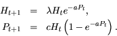
Enhanced Nicholson-Bailey model (ENB) maps current population levels to
future population levels according to
. The
Enhanced Nicholson-Bailey model (ENB) maps current population levels to
future population levels according to
![\begin{displaymath}
\underbrace{a H_t P_t}_{\mbox{\tiny 1 encounter}} + \underbr...
...ny 3 encounters}} + \cdots = H_t\left[ 1 -
e^{-a P_t}\right] .
\end{displaymath}](img144.gif)
There are three fixed points for ENB:
![]() and a mixed
population
and a mixed
population ![]() which must be calculated using a nonlinear root
finder on the equations
which must be calculated using a nonlinear root
finder on the equations
     %
     %   ENB -- a small script for implementing the Enhanced Nicholson Bailey Model
     %

     n=1; a=4; r=1.75; k=1;          % set parameters for ENB
     ngens=50;                       % set number of generations
     h=zeros(1,ngens); p=h;          % initialize population vectors

     p(1)=.1; h(1)=.9;               % set initial conditions

     for t=1:ngens-1                 % iterate ENB for next ngens-1 generations

        h(t+1)=h(t)*exp( r*(1 - h(t)/k) - a*p(t) );
        p(t+1)=n*h(t)*( 1 - exp(- a*p(t) ));

     end                             % of iteration over generations

     plot(h,'b'),hold on, plot(p,'r'),hold off
     legend('host','parasite')
Notice the for and end statements above, which define a loop in
the MATLAB script.
Try running this program for increasingly large ![]() values and see how the dynamics changes.
values and see how the dynamics changes.
EXERCISE 13: The (un-enhanced) Nicholson-Bailey model for host-parasite interactions is
Probably the simplest possible integro-difference equation is one which
incorporates a single step of dispersal followed by a single step of linear,
Malthusian growth at a per-capita rate of ![]() :
:
     %
     %       MALTHUS
     %
     %       matlab code to evaluate dispersal due to convolution
     %       of a spatial dispersal probability with a population density
     %       function.
     %
     %       p(x)    -       population density in x
     %       K(x)    -       probability of individual dispersal to location
     %                          x starting at location 0.
     %       xl	-       maximum x coordinate (also - minimum)
     %       dx	-       spatial step  delta x = 2*xl/np
     %       np	-       number of points  in discretization for x
     %                         (should be a power of 2 for  efficiency of FFT)
     %       c	-       center of spatial  dispersal
     %       D	-       diffusion constant (per step)
     %       r	-       per-capita growth constant
     %

     np=128; xl=5; dx=2*xl/np; c=.4; D=.25;
     r=1.15;
     nsteps=10;

     %
     %       discretize space, define an initial population distribution
     %

     x=-xl+[0:np-1]*dx;
     p=(abs(x+3)<=.5);
     p0=p;           %  keep track of initial population for comparison

     %
     %       define a dispersal kernel
     %

     K=exp(-(x-c).^2/(4*D))/sqrt(4*pi*D);

     %
     %       normalize K to make it have integral one
     %

     K=K/(dx*sum(K));

     %
     %       calculate the fft of K, multiplying by dx to account
     %       for the additional factor of np and converting from a
     %       interval length of 1 to 2*xl.  The fftshift accounts for
     %       using an interval of (-xl,xl) as opposed to (0,2*xl).
     %

     fK=fft(fftshift(K))*dx;

     %
     %       begin iterating the model
     %

     for j=1:nsteps,

     %
     %       calculate the fft of p; perform the convolution
     %

        fp=fft(p);
        fg=fK.*fp;

     %
     %       fg now contains the fourier transform of the convolution;
     %       invert it, multiply by post-dispersal reproduction,
     %        and take a look.
     %

        g=r.*abs(ifft(fg));
        plot(x,p0,'r',x,g,'b'), axis([-xl xl 0 1.6])
        pause(.5)     % pause for .5 sec  to see the plot

     %
     %       update p and move to the next time step
     %
        p=g;

     end     % of the iterations
There are some features to note about this script. The pause(.5)
command causes the program to stop for half a second and plot. Try commenting
out this line and running the program again - you will see only the end
result as opposed to the intervening steps. Now try removing the parentheses,
that is, replace pause(.5) with pause. This will cause the
program to wait for user input before proceeding - for example, just hit the
space bar in the command window and the program will advance one step.
Finally, to see all the steps together, replace the plot line with
hold on, plot(x,p0,'r',x,g,'b'), axis([-xl xl 0 1.6]), hold offThis should allow you to see all the iterations on the same plot, with one additional per each `click' of the space bar.
EXERCISE 14: Imagine now that the net fecundity, ![]() , depends on space - that is,
eggs hatch and survive better in some regions or others. Modify the program
above so that
, depends on space - that is,
eggs hatch and survive better in some regions or others. Modify the program
above so that ![]() is 1.3 for
is 1.3 for ![]() and
and ![]() elsewhere. (Hint:
the MATLAB command ones(1,np) generates a row-vector of ones of length
np and the logical statement (abs(x) <= 1.5) generates a vector
which has elements 0 where
elsewhere. (Hint:
the MATLAB command ones(1,np) generates a row-vector of ones of length
np and the logical statement (abs(x) <= 1.5) generates a vector
which has elements 0 where ![]() and 1 where
and 1 where ![]() ). Will the
population persist in this case? Now try the same scenario with with mean
dispersal distance zero (
). Will the
population persist in this case? Now try the same scenario with with mean
dispersal distance zero (![]() ).
).
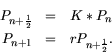
The idea for implementing an IDE approach to known discrete dynamics is to imagine that the behavior of the organisms can be represented in two stages:
![\begin{eqnarray*}
H_{t+1/2}(x,y) = & f(H_t, P_t) &= H_t(x,y) \exp \left[
r \le...
...H_t, P_t) &= n H_t(x,y) \left(
1 - \exp[-aP_t(x,y)]
\right) .
\end{eqnarray*}](img171.gif)
Below appears psuedo-code which implements the above model in MATLAB. For interesting results parameter values are chosen where oscillatory instabilities and chaos occur.
     %
     %       NBSPACE
     %
     %       matlab code to iterate an enhanced Nicholson-Bailey model
     %       for host and parasite, with each capable of diffusive movement.
     %
     %       Intermediate variables (*) are created  using a discrete
     %       enhanced N-B step:
     %
     %              h* = h(t) exp[ r (1 - h(t)/k) - a p(t) ]
     %              p* = n h(t) ( 1 - exp[- a p(t) ] )
     %
     %       This population is then allowed to disperse using a spatial
     %       convolution, * below, (like a long step of  a heat equation):
     %
     %              h(t+1) = p_h(x,y) * h*
     %              p(t+1) = p_p(x,y) * p*
     %
     %       p_h and p_p can be any probability functions representing the
     %       dispersal of the two species; I have used Gaussians below.
     %
     %       Parameters appearing (and their interpretation):
     %
     %              r       reproduction rate of host  species
     %              k       carrying capacity of host species
     %              a       encounter rate or effectiveness of parasite on host
     %              n       parasites produced by a successful infestation
     %
     %       Parameters used for the code:
     %
     %              np       number of points in x, y directions (a power of 2)
     %              xl       length of domain in x and y directions
     %              dx       grid spacing
     %              dt       a time-step length
     %              mu       followed by h and p -- diffusion parameter for each
     %                            species
     %              ngens    number of steps to run the code (number of
     %                            generations

     %
     %       set parameters and spatial grids
     %
     np=64; mup=.02; muh=.02; dt=.5; xl=10; dx=2*xl/np; ngens=20;
     x=linspace(-xl,xl-dx,np);
     y=x; [X,Y]=meshgrid(x,y);

     %
     %       set up spatial parameters
     %

     n=ones(np);
     a=4*ones(np);
     r=1.75*ones(np);
     k=ones(np);

     %
     %       Set up stuff for movie
     %
     % M=moviein(ngens);          %       If you want movies

     %
     %       Set up initial conditions
     %

     p0=.5*(1+cos(.5*pi*X/xl+pi/4*rand(np)).*sin(pi*Y/xl-pi/2*rand(np)));
     h0=.5*rand(np).*(1+cos(4*pi*sqrt(X.^2+Y.^2)/xl));

     %
     %       Define movement kernels for host and parasite
     %

     hker=exp(-(X.^2+Y.^2)/(4*muh*dt))/(4*pi*dt*muh)*dx^2;
     Fhker=fft2(hker);       % FFT is taken because we will use it often,
                             % two factors of dx; one for each dimension

     pker=exp(-(X.^2+Y.^2)/(4*mup*dt))/(4*pi*dt*mup)*dx^2;
     Fpker=fft2(pker);

     %
     %       Now we are in a position to iterate for
     %       a number of generations equal to ngens
     %

     for j=1:ngens

     %
     %       Advance the life cycles using adjusted N-B model
     %

        hn=h0.*exp(r.*(1-h0./k)-a.*p0);
        pn=n.*h0.*(1-exp(-a.*p0));

     %
     %        Do the dispersal step
     %

        fhn=fft2(hn);              %       First take fft of each species
        fpn=fft2(pn);              %       First take fft of each species

     %
     %       Now do the convolutions.
     %       The fftshift serves to center the probability functions.
     %
        h0=real(fftshift(ifft2(Fhker.*fhn)));
        p0=real(fftshift(ifft2(Fpker.*fpn)));

     %
     %       Now plot the solution
     %

        pcolor(X,Y,h0-p0), shading interp, colormap(jet), axis square, colorbar
     % M(:,j) = getframe;         %       If you want movies

     end
     %
     %       Here ends the iteration
     %

     %
     %  To play the movie,  use this command:
     %  movie(M,2,8)
Now, if you want to run this M-file as it stands you should see basically a complicated spatial field at the end. This field is coded so that the difference between relative abundances of host and parasite can be seen; places with more abundant hosts will appear as red, more abundant parasties as blue. To see a movie you must un-comment the
% If you want movies
lines in the script. These movies can be memory-intensive, so don't get
freaked out if your computer suddenly starts whirring, clicking and smoking!
Also, movies are created in MATLAB basically by saving screen-grabs of the
(normally computationally intensive) graphics. This allows the frames of the
movie to be `stacked' together and viewed rapidly, but it also means that you
can not change the size of movie when it is being viewed, and if you pop up
any windows which overlap with the MATLAB graphics window while you are
producing a movie, MATLAB will grab whatever you popped up and keep it in the
movie! (I had a particularly bad moment discovering this making a
movie for a conference. While producing the movie I happened to go lingerie
shopping for my wife at the Victoria's Secret web site.....) The command
movie(M,2,8)
will play the movie, M, 2 times at a speed of 8 frames per second. The
advantage of having a movie is that you can play it again and again without
re-doing the calculation. You can also save a movie to a transportable AVI
file.
EXERCISE 15: Copy the above MATLAB M-file and modify it to implement an IDE for the normal, vanilla Nicholson Bailey model. Run the model with initial conditions which are:
EXERCISE 16: Create a MATLAB M-file which will simulate the spatial spread of a single population satisfying (when space is not included) a logistic model:
One of the nice things about IDE models implemented in MATLAB is that they can
accomodate spatial structure easily. Returning to the ENB model for a moment,
consider the ways in which the spatial environment might influence parameters
in the model. It is possible that motility of organisms can vary with the
environment - an example of this is provided above in the section on
victim-taxis. Neglecting this, the environment can have a plethora of
life-history effects, perhaps the largest of which is alteration in the
`carrying capacity,' ![]() , of the environment for the host. Returning to the
MATLAB code for the ENB given above, notice that when parameters are defined
they are defined as matrices of the same size as all spatial variables.
When the parameters are used in the life-history step of the IDE, the MATLAB
implementation accounts for element-by-element matrix multiplication.
Consequently, if we wanted to simpulate the effect of a crop on the host, we
could insert
, of the environment for the host. Returning to the
MATLAB code for the ENB given above, notice that when parameters are defined
they are defined as matrices of the same size as all spatial variables.
When the parameters are used in the life-history step of the IDE, the MATLAB
implementation accounts for element-by-element matrix multiplication.
Consequently, if we wanted to simpulate the effect of a crop on the host, we
could insert
     k=.1*ones(np)+(abs(X)<=.25)+(abs(X)>=1.75 & abs(X)<=2.25)...
        +(abs(X)>=3.75 & abs(X)<=4.25)...
        +(abs(X)>=5.75 & abs(X)<=6.25)...
        +(abs(X)>=7.75 & abs(X)<=8.25)...
        +(abs(X)>=9.75 & abs(X)<=10.25);
in place of the existing line
k=ones(np)
(Notice the MATLAB form of `continuation' for a long line: the ellipsis `...')
This will have the effect of putting `stripes' of
high carrying-capacity crops in the environment.
EXERCISE 17: Implement the crop-structured spatial heterogeneity indicated above. Think of a way to introduce parameters so that the width of the crop stripes and their relative `value' to the host are easy to adjust. Try some simulations - are there `crops' and spatial structures which are more or less vulnerable to infestation by the host even in the presence of the parasite?
EXERCISE 18: Suppose that the cropping structure also influences the `efficiency,'
![]() , of the parasite. How should this be included, and what are its effects
on the dynamics?
, of the parasite. How should this be included, and what are its effects
on the dynamics?
Although they may be tedious, artificial spatial structures are much easier to introduce than `natural' ones, just because a semi-structured `random' environment is very hard to put together off the top of your head. Of course, in principle one could take field measurements of a spatial arena and then scan these into density plots, but probably that is beyond the scope of our current lab experience. One alternative was suggested to me by Professor Jon Allen (Department of Entomology and Nematology, University of Florida, Gainesville). The following MATLAB script, named `rockies.m' generates a randomized but spatially correlated structure by choosing random phases and angles in Fourier spectrum, but using a user-specified power law for decreasing energy in the power spectrum. (If this doesn't make sense to you, don't sweat it; the program will work anyway). The MATLAB script requires a `fractal dimension', H, which increases the spatial correlation (think regularity) as the `dimension' increases. The code appears below, but is available for download in the class directory. The script will produce a surface plot of the field B, which is normalized so that its peak value is one, and is also then available to be used for simulating resource heterogeneity. The `power-law' decrease in the spectral energy of waves, p, is defined as p=(H+1)/2 because when the exponent is 1/2 the distribution is theoretically indistinguishable from `white' noise. The most interesting structures appear for H between .5 and 1.5.
     %
     %		ROCKIES
     %
     % 	This cryptic matlab script generates a structured but random spatial
     % 	environment of size NxN.  The user inputs the following:
     %     N - number of grid points in both x,y directions
     %     H - fractal dimension (the bigger this is the smoother the landscape)
     %

     N=64; H=1;
     p=(H+1)/2;

     [I,J]=meshgrid([-N/2+1:N/2], [-N/2+1:N/2]); % wave modes
     randn('seed',0);
     phases=2*pi*rand(N);                % random phases
     amp=randn(N).*(I.^2+J.^2).^(-p);    % normal  amplitudes about power law
     amp(N/2,N/2)=0;                     % mean amp of zero
     fA=amp.*exp(i*phases);              % field in tranform space

     A=ifft2(fA);                        % invert transform
     B=abs(A);                           % make field real
     B=B/max(max(B));                    % normalize

     surf(B), colormap(jet), shading interp
     title(['Log(PS) = - ',num2str(p),' k'])
     view(-37.5,60)
EXERCISE 19: Download the program rockies.m and run it for a few choices of the `fractal dimension.' Describe the relationship between increasing this parameter and the output field.
EXERCISE 20: Use the B field output by the rockies program to generate random landscapes of carrying capacity for the ENB model. One way to do this would be simply to execute the rockies script and then state
k=2*B;
in the ENB program. Modify the graphic output to include contours of the
resource with the density plots of the relative abundance of
victims/parasites. What dynamics behaviors seem to correlate with what
landscape features? What consequences do you think this might have for
Nicholson's hypothesis for the persistence of parasitized populations in
space?
Wow, Good Job! You now know secret and official things about the computational implementation of IDE using MATLAB !